Image Captioning to describe images automatically | Blogs

Introduction

Automatically describing the content of an image is a common problem in Artificial Intellligence that connects computer vision and natural language processing. Here we will learn about a generative model based on deep recurrent architecture that combines the recent advancements in computer vision and natural language processing. The model in the end will be able to generate the target description sentence when inputs the image. We will also discuss beam search strategy to get the best caption out of many caption. Also we will learn about BLEU score which is common metric for machine translation tasks.

Here, I will be discussing 'merge' architecture to generate Image Captions which is different from the tradtional views of Image Captioning where image features are 'injected' in the RNN. Please read the following two papers to get understanding of 'injected' architecture.

Vinyals, Oriol, et al. Show and tell: A neural image caption generator. CVPR, 2015.
Xu, Kelvin, et al. Show, attend and tell: Neural image caption generation with visual attention. ICML, 2015.

The idea of 'merge' architecture is taken from the following paper. This is an architecture which is different from the dominant view in the literature. Here, the RNN is viewed as only encoding the previously generated words. This view suggests that the RNN should only be used to encode linguistic features and that only the final representation should be ‘merged’ with the image features at a later stage. Here I it is called 'merge' architecture.

What is the Role of Recurrent Neural Networks (RNNs) in an Image Caption Generator?

Model Architecuture

The diagram below shows the whole attention model in one view.

This architecture keeps the encoding of linguistic and perceptual features separate, merging them in a later multimodal layer, at which point predictions are made. In this type of model, the RNN is functioning primarily as an encoder of sequences of word embeddings, with the visual features merged with the linguistic features in a later, multimodal layer. This multimodal layer is the one that drives the generation process since the RNN never sees the image and hence would not be able to direct the generation process.

In this model, RNN is only used as language model. RNN is feeded the word embeddings of partial caption starting from special token 'seq_start', the RNN then generate encoded representation of partial sequence. While CNN which is generally pretrained for image classification task like imagenet is feeded the image, which gives a image representation of that image. We can use VGG, Inception or resnet as pretrained CNN. These two representation i.e. language feature and image feature are appended together and feeded into another Feed Forward neural network. This Feed Forward Neural Network will output a vector of size equal to size of vocabulary. Index of highest value in that vector represents the next word of caption which is combined with the partial caption and again process continues untill we get the 'seq_end' token from FNN.

Building Image Caption Generator

Firstly, get a dataset which has image and its corresponding captions. There are many such dataset available online. Some famous ones are flickr8k, flickr30k or Microsoft COCO dataset. We will use flickr8k dataset which is easily available online. It has 8k images with 5 captions for each image.

Now, preprocess these captions like remove non alphabet characters, make everything in lower case, remove dangling characters. After that append sequence start and sequence end word at the begining of caption and at the end. We will use <S> as seq start and </S> as seq end. Now form a dictionary out of all words present in all captions combined which will point out some index. Similary create a reverse dictionary which point word from index. Decide a max length of a sequence which ideally should be equal to number of words in biggest caption.

Now we will build the training dataset. Select a caption, split it, take its first word and pre pad it to length of max sequence length this will be your x and its corresponding target will be second word. Repeat this for max seq length or length of caption, include next word in x and next word as target. Repeat this for all captions. Also remember the corresponding image of that caption.

Example: Caption: <S> red car on road. </S>
Say max seq length is 5
x: [0,0,0,0,<S>] y: red
x: [0,0,0,<S>,red] y: car
x: [0,0,<S>,red,car] y: on
x: [0,<S>,red,car,on] y: road
x: [<S>,red,car,on,road] y: </S>

We will convert our target y to one hot encoded representation and x to seq with words denoted by their index. Now use any pretrained CNN used for image classification task such as imagenet and take out image feature from the last dense layer. Here for example we have used VGG19 and taken out 4096 length image feature from last dense layer. Create a model which take seq as input and use embedding layer to get a embedding of that sequence, we can use pretrained embedding like glove also. Now append this embedding of seq and image feature. And pass it though a feed forward neural network whose last layer is of size of VOCAB. This last layer denotes the probability of each word. Take out the word with highest probability and this will be the next word of seq.

Here is Github Link for full Code

Beam Search

The 'merge' model described above output a probability distribution over each word in the vocabulary for each word in the output sequence. It is then left to a decoder process to transform the probabilities into a final sequence of words. The final layer in the neural network model has one neuron for each word in the output vocabulary and a softmax activation function is used to output a likelihood of each word in the vocabulary being the next word in the sequence. Candidate sequences of words are scored based on their likelihood. It is common to use a greedy search or a beam search to locate candidate sequences of text.

Greedy Search Decoder

Each individual prediction has an associated score (or probability) and we are interested in output sequence with maximal score (or maximal probability). One popular approximate technique is using greedy prediction, taking the highest scoring item at each stage. While this approach is often effective, it is obviously non-optimal. Indeed, using beam search as an approximate search often works far better than the greedy approach.

Beam Search Decoder

Instead of greedily choosing the most likely next step as the sequence is constructed, the beam search expands all possible next steps and keeps the k most likely, where k is a user-specified parameter. At each step, all the successors of all k states are generated. If any one is a goal, the algorithm halts. Otherwise, it selects the k best successors from the complete list and repeats.

Larger beam widths result in better performance of a model as the multiple candidate sequences increase the likelihood of better matching a target sequence. This increased performance results in a decrease in decoding speed. The search process can halt for each candidate separately either by reaching a maximum length, by reaching an end-of-sequence token, or by reaching a threshold likelihood.

Probabilities are small numbers and multiplying small numbers together creates very small numbers. To avoid underflowing the floating point numbers, the natural logarithm of the probabilities are multiplied together, which keeps the numbers larger and manageable. Further, it is also common to perform the search by minimizing the score, therefore, the negative log of the probabilities are multiplied. This final tweak means that we can sort all candidate sequences in ascending order by their score and select the first k as the most likely candidate sequences.

Example

In the above task one solution is to always pick the most probable word and add it to the prefix. This is called a greedy search and is known to not give the optimal solution. The reason is because it might be the case that every combination of words following the best first word might not be as good as those following the second best word. We need to use a more exploratory search than greedy search.

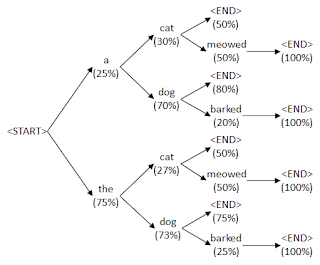
The tree shows a probability tree of which words can follow a sequence of words together with their probabilities. To find the probability of a sentence you multiply every probability in the sentence's path from to . For example, the sentence "the dog barked" has a probability of 75% × 73% × 25% × 100% = 13.7%. The problem we want to solve is how to find the sentence that has the highest probability.

One way to do this is to use a breadth first search. Starting from the node, go through every node connected to it, then to every node connected to those nodes and so on. Each node represents a prefix of a sentence. Of course a breadth first search is impractical on any language model that has a realistic vocabulary and sentence length since it would take too long to check all the prefixes in the tree. We can instead opt to take a more approximate approach where we only check a subset of the prefixes. The subset would be the top 10 most probable prefixes found at that point. We do a breadth first search as explained before but this time only the top 10 most probable prefixes are kept and we stop when the most probable prefix in these top 10 prefixes is a complete sentence.

BLUE Score

BLEU, or the Bilingual Evaluation Understudy, is a score for comparing a candidate translation of text to one or more reference translations. A perfect match results in a score of 1.0, whereas a perfect mismatch results in a score of 0.0.

The primary programming task for a BLEU implementor is to compare n-grams of the candidate with the n-grams of the reference translation and count the number of matches. These matches are position-independent. The more the matches, the better the candidate translation is. Unfortunately, MT systems can overgenerate “reasonable” words, resulting in improbable, but high-precision, translations. Intuitively the problem is clear: a reference word should be considered exhausted after a matching candidate word is identified. We formalize this intuition as the modified unigram precision.

We first compute the n-gram matches sentence by sentence. Next, we add the clipped n-gram counts for all the candidate sentences and divide by the number of candidate n-grams in the test corpus to compute a modified precision score, pn, for the entire test corpus.

The BLEU metric ranges from 0 to 1. Few translations will attain a score of 1 unless they are identical to a reference translation. For this reason, even a human translator will not necessarily score 1.

NLTK provides the sentence_bleu() function for evaluating a candidate sentence against one or more reference sentences. NLTK also provides a function called corpus_bleu() for calculating the BLEU score for multiple sentences such as a paragraph or a document.

A Discussion on BLEU Score