In NLP application we have to work with texual data. Well we can't directly feed our textual data for training into our ML models, Deep Learning Models etc. Let it be regression, classification or any NLP task, we need to convert our textual data into numerical form that can be feeded into models for futher processing.

Word Embedding converts textual data into numerical data of some form. In general, word embedding convert a word into some sort of vector representation.

Now, we will broadly classify word embedding in 2 types and then dive deep into their types

1. Frequency based Embedding

   • Count Vector
   • Tf-Idf Vector

2. Prediction based Embedding

   • CBOW (Continous Bag of Words)
   • Skip-Gram

1. Frequency based Embedding

These are the very basic, easy and fast method to word vectors. These work on the basis of count of word in each document. It can be Count Vector, Tf-Idf vector, or Co-Occurance vector. We will discuss here only Count vector and Tf-Idf vector.

1.1 Count Vector

Lets us understand this by looking into a simple example. Lets take two documents

d1 = "Take a look into the beauty of the word embedding."
d2 = "The word vectorizer is the most basic word embedding"

There are 12 unique words, So here our word vector will be of size 12, which means each word can be denoted by a vector of size 12.

Lets, arrange all unique words in alphabetic order. That would be "basic, beauty, embedding, into, is, look, most, take, the, vectorizer, word".

Now lets prepare a dictionary where each word is mapped with index in vector.
{'basic': 0,'beauty': 1,'embedding': 2,'into': 3,'is': 4,'look': 5,'most': 6,'of': 7,'take': 8,'the': 9,'vectorizer': 10,'word': 11}

So, suppose we want to denote a word by vector.
vectorizer = [0, 0, 0, 0, 0, 0, 0, 0, 0, 0, 0, 1]

Lets convert both our sentence into vector.

	basic	beauty	embedding	into	is	look	most	of	take	the	vectorizer	word
d1	0	1	1	1	0	1	0	1	1	2	0	1
d1	1	0	1	0	1	0	1	0	0	2	1	2

above is given vector representaion of documents d1 and d2
Here is the example code, to form count vector using sci-kit library
>>> from sklearn.feature_extraction.text import CountVectorizer
>>> text = ["Take a look into the beauty of the word embedding.","The word vectorizer is the most basic word embedding"]
>>> cv = CountVectorizer()
>>> cv.fit(text)
>>> text_vector = cv.transform(text)
>>> text_vector.toarray()
array([[0, 1, 1, 1, 0, 1, 0, 1, 1, 2, 0, 1],
[1, 0, 1, 0, 1, 0, 1, 0, 0, 2, 1, 2]])
>>> cv.vocabulary_
{'basic': 0,
'beauty': 1,
'embedding': 2,
'into': 3,
'is': 4,
'look': 5,
'most': 6,
'of': 7,
'take': 8,
'the': 9,
'vectorizer': 10,
'word': 11}


1.2 TF-IDF Vector

It is another method which also based on the frequency of words in documents. But overcome some flaws of countvectorizer. It takes into account not only frequency of word in each document but also entire corpus.

Some words like 'the','a','is','that' appear more often then other words in every document. These word doesn't seem to change the sentiment of sentence. So we would like to weight down the words which occur quite often in most of the documents.

For documents,
d1 = "Take a look into the beauty of the word embedding."
d2 = "The word vectorizer is the most basic word embedding"

Lets look what Tf-Idf does,
TF = ( Freq of word in a document ) / ( No of words in that documents )
TF(take,d1) = 1/10 = 0.1
TF(the,d2) = 1/9 = 0.11

IDF = log( No of docs / No of docs term t has appeared ) #without smoothing
where
IDF(the) = log(2/2) = 1
IDF(take) = log(2/1) = 0.6931


TF-IDF(take,d1) = tf*idf = 0.1*0.6931 = 0.0693

sci-kit learn library uses TF-IDF which by default takes smoothing factor into account so values might be different.
>>> from sklearn.feature_extraction.text import CountVectorizer
>>> text = ["Take a look into the beauty of the word embedding.","The word vectorizer is the most basic word embedding"]
>>> cv = CountVectorizer()
>>> cv.fit(text)
>>> text_vector = cv.transform(text)
>>> text_vector.toarray() array([[0, 1, 1, 1, 0, 1, 0, 1, 1, 2, 0, 1], [1, 0, 1, 0, 1, 0, 1, 0, 0, 2, 1, 2]])
>>> cv.vocabulary_ {'basic': 0, 'beauty': 1, 'embedding': 2, 'into': 3, 'is': 4, 'look': 5, 'most': 6, 'of': 7, 'take': 8, 'the': 9, 'vectorizer': 10, 'word': 11}


Pros:

• It is very easy and fast method to perform word embeddings.

Cons:

• If the vocabulary is too large then the spase matrix created will be too large and will take a lot of memory. Also processing that huge matrix will be a burden.

2. Prediction Based Vector

To overcome the limitations of previous methods of representation. Another method is introduced which with the help of 1-Hidden Layer Neural Network forms a N-dimensional representation of word called word vector.

These are great for many NLP task like word analogies and word similarities.
They can also perform task like King-Man+Woman = Queen

Lets take a look at 2 techniques to generate word vectors.

2.1 CBOW (Continuous Bag of Words)

It works by finding or predicting the probability of a word in a given context. A context is a group of words. Given the context, we will predict the target word.

We will use neural network with 1-hidden layer whose size is equal to the size of word embedding we want.
Suppose, we have a vocabulary of size V, embedding size of N and context size of C. So architecture of neural network will be as follows:
As shown in figure above, Input layer have multiple vectors given as input. These vectors are one hot encoded vectors. These multiple vectors belongs to each word in context. Hidden layer size is equal to embedding size. While output layer is a one hot encoded target word.

Objective function is Negative log likelihood of a word i.e. -log(p(wo/wi)) where,
wo : output words, wi : context words

Each word will be represented by a vector of size N i.e. Hidden Layer.

2.2 Skip-Gram

This is somewhat similar to CBOW, input is target word and the outputs are word surrounding target i.e. context. For example in sentence "I have a cute dog.". If input is "cute" then output is "I", "have", "a", "dog" assuming window size of 5.

Similar to CBOW, it contain 1 hidden layer of size equal to embedding size.
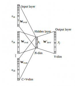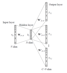As shown in figure above, Input layer have target one hot encoded work vector given as input. Hidden layer size is equal to embedding size. While output layer is a one hot encoded context words.

Vectors are "meaningful" in terms of describing the relationship between words. The vector obtains by subtracting two related words sometimes express a meaningful concept such as gender or verb tense.

Pros:

• Word Vectors take less memory than previous word embedding methods.
• Word Vectors can be used to describe similarity between words using cosine similarity.
• Many library are already present like Gensim, Glove, Spacy which helps us to deal with Word vectors.

Cons:

• Training for CBOW or Skip-Gram can take so much processing beacause of large vocabulary size.

Lets look at an example to build word vectors by using Gensim Library.
import gensim.models.word2vec as w2v
import numpy as np
sentence_tokens = np.array([["This","is","a","game","of","thrones","books","corpus"],
["You","can","select","any","corpus"],
["You","must","convert","corpus","in","this","form"]])
embedding_size = 300 #size of embedding
min_word_count = 3 #word must appear atleast 3 times
num_workers = multiprocessing.cpu_count() #using multiple processors
context_size=7 #looking at 7 words at a time
downsampling = 1e-3 #Downsample setting for frequent words

thrones2vec = w2v.Word2Vec(
sg=1, #1 skip-gram 0- CBOW
seed=seed,
workers= num_workers,
size = num_features,
min_count = min_word_count,
window = context_size,
sample = downsampling
)

thrones2vec.build_vocab(sentence_tokens)
#start training, this might take time
thrones2vec.train(sentence_tokens,
total_examples=len(sentence_tokens),
epochs=25
)
thrones2vec.save("thrones2vec.w2v") #to save word2vec model
thrones2vec = w2v.Word2Vec.load("thrones2vec.w2v") #to load word2vec model


Lets look at some applications of word2vec.
>>> thrones2vec.wv.vectors #gives V*N dimensional matrix
>>> thrones2vec.wv.vocab #gives list of words of size V
>>> thrones2vec.wv.most_similar("stark")
[('eddard', 0.6009404063224792),
('snowbeard', 0.4654235243797302),
('accommodating', 0.46405118703842163),
('divulge', 0.4528692960739136),
('edrick', 0.43332362174987793),
('interred', 0.4253771901130676),
('executed', 0.42412883043289185),
('winterfell', 0.4224868416786194),
('shirei', 0.4207403063774109),
('absently', 0.419999361038208)]
>>> #Finding the degree of similarity between two words.
>>> thrones2vec.wv.similarity('woman','man')
0.73723527
>>> #Finding odd one out.
>>> thrones2vec.wv.doesnt_match('breakfast cereal dinner lunch';.split())
'cereal'
>>> #Amazing things like woman+king-man =queen
>>> thrones2vec.wv.most_similar(positive=['woman','king'],negative=['man'],topn=1)
queen: 0.508
>>> #Probability of a text under the model
>>> thrones2vec.wv.score(['The fox jumped over the lazy dog'.split()])
0.21
>>> def nearest_similarity_cosmul(start1, end1, end2):
.........similarities = thrones2vec.wv.most_similar_cosmul(
.........positive=[end2, start1],
.........negative=[end1])
.........start2 = similarities[0][0]
.........print("{start1} is related to {end1}, as {start2} is related to {end2}".format(**locals()))
>>> nearest_similarity_cosmul("stark", "winterfell", "riverrun")
'stark is related to winterfell, as tully is related to riverrun'
>>> nearest_similarity_cosmul("arya", "nymeria", "drogon")
'arya is related to nymeria, as dany is related to drogon'


More Resources

1. Word Embedding tutorials by Analytics Vidhya
2. Skip Gram in detail by Towards Data Science