Policy Gradient and Actor-Critic Algorithm
Contents
- Policy Gradient (REINFORCE)
- Actor-Critic Algorithm:
- Advantage Actor-Critic (A2C)
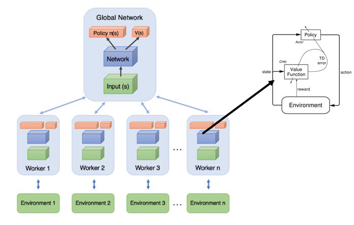
- Asynchronous Advantage Actor-Critic (A3C)
Today most successful reinforcement algorithm A3C, PPO etc belong to the policy gradient family of algorithm often more specifically to the actor-critic family. But before going into mathematics of these algorithm, you must have basic knowledge of Deep Q Learning(below link).
Deep Q Learning
Before going any further, let's understand some drawbacks of Q Learning.
1. The policy implied by Deep Q-Learning is deterministic. This means Q-Learning can't learn stochastic policies, which can be useful in some environments. It means we also need to create our own exploration strategies.
2. There is no way to handle continuous action spaces in Q-Learning. In policy gradient handling continuous action spaces is relatively easy.
3. In policy gradient we are calculating the gradient of policy itself. By contrast Q-Learning we are improving value estimates of different actions in a state, which implicitly improves policy. Improving policy directly is more efficient.
Let's call `\pi \theta(a|s)` the probability of taking action a in state s. `\theta` represents parameters of policy (the weights of Neural Network). The goal is to update `\theta` to values that make `\pi \theta` the optimal policy. `\theta_t` represent the values of `theta` in iteration t. We want to find out the update rule that takes use from `\theta_t` to `\theta_{t+1}` to optimize our policy.
For a discrete action space we will use neural network with softmax output unit, so that output can be thought of as a probability of taking each action in state. Clearly, if action `a^\star` is optimal action, we want `\pi\theta(a^\star | s)` as close to 1 as possible. For this we can simply perform an gradient ascent to update `\theta` in the following way:
$$ \theta_{t+1} = \theta_t + \alpha \nabla \pi_{\theta_t}(a^\star|s) $$
We can view `\nabla \pi \theta_t(a^\star|s)` as direction in which we must move `\theta_t` to increase value of `\pi\theta(a^\star | s)`. Note we are using gradient ascent to increase a value. Thus one way to view this update is that we keep “pushing” towards more of action `a^\star` in our policy, which is indeed what we want.
Of course, in practice, we won’t know which action is best… After all that’s what we’re trying to figure out in the first place! To get back to the metaphor of “pushing”, if we don’t know which action is optimal, we might “push” on suboptimal actions and our policy will never converge. One solution would be to “push” on actions in a way that is proportional to our guess of the value of these actions. We will call our guess of the value of action a in state s Q̂(s,a). We get the following gradient ascent update, that we can now apply to each action in turn instead of just to the optimal action:
$$ \theta_{t+1} = \theta_t + \alpha \hat Q_t(s,a) \nabla \pi_{\theta_t}(a|s) $$
Of course, in practice, our agent is not going to choose actions uniformly at random, which is what we implicitly assumed so far. Rather, we are going to follow the very policy `\pi\theta` that we are trying to train! This is called training on-policy. There are two reasons why we might want to train on-policy:
1. We accumulate more rewards even as we train, which is something we might value in some contexts.
2. It allows us to explore more promising areas of the state space by not exploring purely randomly but rather closer to our current guess of the optimal actions.
This creates a problem with our current training algorithm, however: although we are going to “push” stronger on the actions that have a better value, we are also going to “push” more often on whichever actions happen to have higher values of πθ to begin with (which could happen due to chance or bad initialization)! These actions might end up winning the race to the top in spite of being bad. This means that we need to compensate for the fact that more probable actions are going to be taken more often. How do we do this? Simple: we divide our update by the probability of the action. This way, if an action is 4x more likely to be taken than another, we will have 4x more gradient updates to it but each will be 4x smaller.
$$ \theta_{t+1} = \theta_t + \alpha \frac{\hat Q_t(s,a) \nabla \pi_{\theta_t}(a|s)}{\pi_\theta(a|s)} $$
Now, we can write `\frac{\nabla \pi_{\theta_t}(a|s)}{\pi_\theta(a|s)}` as `\nabla_\theta log \pi_theta(s|a) ` and using return `v_t` as an unbiased sample of `\hat Q_t(s,a)`.
$$ \theta_{t+1} = \theta_t + \alpha v_t \nabla_\theta log \pi_\theta(s|a) $$
A widely used variation of REINFORCE is to subtract a baseline value from the return `v_t` to reduce the variance of gradient estimation while keeping the bias unchanged (Remember we always want to do this when possible). As it turns out, REINFORCE will still work perfectly fine if we subtract any function from Q̂(s,a) as long as that function does not depend on the action. This means that using the  function instead of the Q̂ function is perfectly allowable. For example, a common baseline is to subtract state-value from action-value, and if applied, we would use advantage A(s,a) = Q(s,a) – V(s) in the gradient ascent update.
$$ \theta_{t+1} = \theta_t + \alpha \hat A_t(s|a) \nabla_\theta log \pi_\theta(s|a) $$
where,
`A_t(s,a) = R_t - b` (Return - baseline)
`\pi_\theta(s|a) = policy`
Until now we have studied Critic-only methods and Actor-only methods. Critic-only methods that use temporal difference learning have a lower variance in the estimates of expected returns. A straightforward way of deriving a policy in critic-only methods is by selecting greedy actions actions for which the value function indicates that the expected return is the highest. Actor-only methods (example Policy Gradient) typically work with a parameterized family of policies over which optimization procedures can be used directly. In actor-critic spectrum of continuous actions can be generated, but the optimization methods used (typically called policy gradient methods) suffer from high variance in the estimates of the gradient, leading to slow learning.
Actor-critic methods combine the advantages of actor-only and critic-only methods. While the parameterized actor brings the advantage of computing continuous actions without the need for optimization procedures on a value function, the critic’s merit is that it supplies the actor with low-variance knowledge of the performance. More specifically, the critic’s estimate of the expected return allows for the actor to update with gradients that have lower variance, speeding up the learning process. Actor-critic methods usually have good convergence properties, in contrast to critic-only methods.
In Actor-only policy gradient method we were reducing variance and increasing stability by subtracting the cumulative reward by a baseline. Intuitively, making the cumulative reward smaller by subtracting it with a baseline will make smaller gradients, and thus smaller and more stable updates.
$$ \theta_{t+1} = \theta_t + \alpha \hat Q_t(s|a) \nabla_\theta log \pi_\theta(s|a) $$
As we know, the Q value can be learned by parameterizing the Q function with a neural network.
This leads us to Actor Critic Methods, where:
1. The “Critic” estimates the value function. This could be the action-value (the Q value) or state-value (the V value).
2. The “Actor” updates the policy distribution in the direction suggested by the Critic (such as with policy gradients).
and both the Critic and Actor functions are parameterized with neural networks. In the derivation above, the Critic neural network parameterizes the Q value — so, it is called Q Actor Critic.
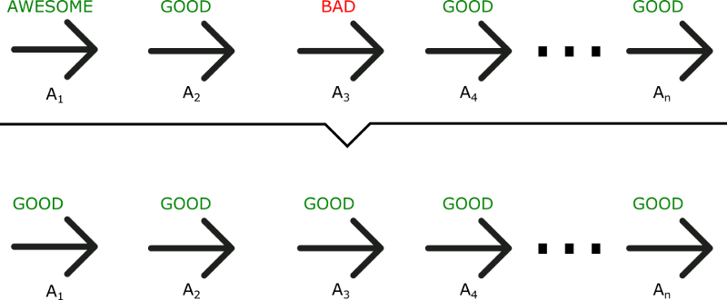 As we can see in this example, even if A3 was a bad action (led to negative rewards), all the actions will be averaged as good because the total reward was important. As a consequence, to have an optimal policy, we need a lot of samples. This produces slow learning, because it takes a lot of time to converge. What if, instead, we can do an update at each time step? The Actor Critic model is a better score function. Instead of waiting until the end of the episode as we do in Monte Carlo REINFORCE, we make an update at each step (TD Learning).