Before we go ahead and start discussing about monte carlo and temporal difference learning for policy optimization, I think you must have knowledge about the policy optimization in known environment i.e. Value Iteraions and Policy Iterations. My advice is to check out the below article to learn about Markov Decision Process, Value Iterations and Policy Iterations.

Policy Optimization in Reinforcement Learning.

Policy Iterations and Value Iterations are algorithms based on dynamic programming which requires knowledge of complete MDP where all environment variables are known. Here the goal of agent was to learn a policy. This problem is called as a Model-Based Learning.

But in real scenerios we do not have knowledge of environment and we have to learn about the environment by experimenting or interacting with the environment. This problem is called Model Free Learning.

1. We will miss a transition model, so we don't have know what's going to happen after each action we take before hand.
2. We will also miss our reward function.

Exploitation vs Exploration

This applies to system that want to aquire new knwoledge and maximize their reward at the same time.
Example. Think of a slot machine in casino. Each machine has its own probability of winning. As a player you want to make as much money as possible. Here's the dilemma. How do you figure out which of the machine have best odds, while at the same time maximizing your profit? If you constantly played one of the machines you would never gain any knwoledge about the odds of other machine. Also if you always picked a machine at random you would learn a lot about other machines at random you would learn a lot about other machines bit probably wouldn't make as much as money as could have always playing "best machine".

This applies to principle of our choices in lives. Do we try drastically different things to explore that what makes us happy, or do we exploit our current situation and knowledge to make the best out of it? In today's society we are loosely based on what is called epsilon-decreasing startegy. Epsilon decreases over time, we try to figure out what we want to do at young age, and then stick with it throughout our lives. Is this strategy optimal? or it is imposed on us by the society.
In slot machine example we wanted to make as much money as possible. This was matrix we tried to optimize. In real life example matrix is how much money we make? How much free time we have? How safe family is?

Let's look at some strategies which can help us with this dilemma.

1. Epsilon-decreasing with softmax

We exploit the current situation with the probability 1-epsilon and explore a new option with the probability epsilon, with epsilon decreasing over time. In case of exploring we dont't want to just pick each option at random, instead we estimate the outcome of each option and then pick based on that (softmax part).

2. Upper confidence bound strategy

We always pick the option with highest possible outcome, even if that outcome is very unlikely. The intuition behind this stategy is that options with high uncertainity unsually lead to a lot of new knowledge. We don't know enough about option to accurately estimate the return and by pursuing the option we are bound to learn more and improve our future estimation. In simulated settings this algorithm does well when we have many options with differet variances.

3. Contextual-Epsilon-greedy strategy

Similar to epsilon-greedy, but we choose the value of epsilon based on how critical our situation is. When we are in critical situation (large debt, need to provide for a sick family) we always exploit instead of explore-we do what we know works well. If we are in situation that is not critical we are more likely to explore new things. This strategy makes intuitive sense, but I believe that is not commonly followed. Even in non-critical situations we often choose to keep doing what we have always done due to our risk-averse nature.

4. Optimistic Initialization

This is an simple and practical idea. Initialize everything as everything is highly rewarding. We will assume that a action in a state is highly rewarding untill proven otherwise. This methods gives chance to every state-action pair to prove itselt. But it could take a lot of time since we now need to try and explore every state-action pair to know its exact value.

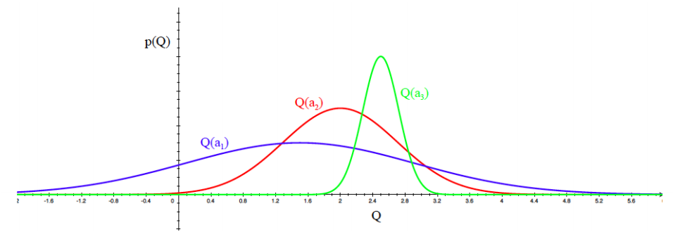
5. Optimism in the face of uncertainity

In this we will always pick the action which have a chance of being highly rewarding. Let's understand this with a simple example below.
Here, what action should we pick? The more uncertain we are about an action value. The more important is to explore an action. It could turn out to be the best action.
Here we will pick the blue action as it seems to be highly rewarding however it very less unlikely that red action.

Monte Carlo Methods :

Monte Carlo methods are large family of compuational algorithms that rely on random sampling. These methods are mainly used for numerical integration, stochastic optimization, character distributions etc.

Monte Carlo vs Dynamic Programming:
1. No Need of Complete Markov Decision process.
2. Computatinally More efficient.
3. Can be used with stochastic simulators.

In reinforcement learning for a unknown MDP environment or say Model Free Learning. Monte Carlo will learn directly from the epsiode of experience. MC uses simplest possible idea value of a state-action pair is mean of all returns.
Goal: Learn `V_{\pi}` from episode of experience.
Return: Return is total discounted reward ` G = R_{t+1} + \gamma R_{t+2} +....+ \gamma^{t-1}R_{T} `
Value Function: Value function is expected return ` V_{\pi}(s) = E_{\pi} [ G_{t} | S_{t}=S ] `

MC uses emperical mean return instead of expected return.

There are 2 types of Monte Carlo Control Methods
1. On-policy First Visit Monte Carlo Control : In each episode, we will consider only first visit of every state-action pair to calculate the mean return.
2. On-policy Every Visit Monte Carlo Control : In each episode, we will consider every visit of every state-action pair to calucalte the mean return. Here we will discuss First Visit Monte Carlo Control only.

Algorithm for First Visit Monte Carlo Control:

• Initialize for all s `\in`, a `\in` A(s):
• • Q(s,a) `\leftarrow` arbitary
  • Visit(s,a) `\leftarrow` 0
  • `\pi`(a|s) `\leftarrow` an arbitary `\epsilon` soft policy
• Repeat Forever
• Generate an episode using `\pi`
  For each pair s,a appearing in the episode
  • G `\leftarrow` the return the follows first occurence of s,a
  • Visit(s,a) `\leftarrow` Visit(s,a) + 1
  • Q(s,a) `\leftarrow` Q(s,a) + 1/Visit(s,a) (G - Q(s,a)) #this is the incremental mean
• For each S in episode
  • `A^\ast \leftarrow argmax_a Q(s,a) `
  • For all `a \in A(s)`:
    $$ \begin{equation} \pi(a,s) = \left \{ \begin{aligned} &max(A^\ast(s,a)), && \text{if } \text{random} > \epsilon \\ &\text{random}(A(s)), && \text{otherwise } \end{aligned} \right. \end{equation} $$

Code for First Visit Monte Carlo Control to solve Frozen Lake OpenAI gym game:

Temporal Difference Learning

It is a combination of Monte Carlo Learning and Dynamic Programming. Just like Monte Carlo, Temporal Difference method also learn directly from the episodes of experience. But in contrast to Monte Carlo Learning, Temporal Difference learning will not wait till the end of episode to update expected future rewards estimation(V), it will wait only until the next time step to update value estimates.

In Monte-carlo: $$ V(S_t) \leftarrow V(S_t) + \alpha \Big( G_t - V(S_t) \Big) $$
In Temporal Difference: $$ V(S_t) \leftarrow V(S_t) + \alpha \Big( R_{t+1} + \gamma V(S_{t+1}) - V(S_t) \Big) $$
Where,
` R_{t+1} + \gamma V(S_{t+1}) ` is estimated return or TD target
` \partial_t = R_{t+1} + \gamma V(S_{t+1}) - V(S_t) ` is called TD error

Temporal Difference is generally more effective thatn Monte Carlo. It is more sensitive to intial value. Temporal Difference Control Learning has 2 alogrithm.
1. SARSA (On policy TD control)
2. Q Learning (Off policy TD control)

Let's discuss On-policy learning and Off-policy learning before going into these algorithms.
On-policy Learning : On policy learning method , means it uses the same policy to choose the next action A'. Learn about the policy `\pi` from the experience sampled from `\pi`.
Off-policy Learning : Off policy learning method , means, it uses the target policy (greedy) to choose the best next action A' while following the behavior policy (epsilon-greedy).

SARSA (state-action-reward-state-action)

$$ Q(S,A) \leftarrow Q(S,A) + \alpha \Big( R + \gamma Q(S',A') - Q(S,A) \Big) $$
The agent starts in state S, performs action A, and get reward R and goes to state S' and chooses action A' there and then update the value of A' in S. Here TD target is ` R + \gamma Q(S',A') ` and TD error is ` R + \gamma Q(S',A') - Q(S,A) `

Algorithm for SARSA : An On-policy TD control Algorithm :

• Initialize `Q(s,a) \forall s \in S, a \in A(S) arbitarily and Q`(terminal) = 0
• Repeat (for each episode):
• • Initialize S
  • Choose A from S using policy derived from `Q(\epsilon-greedy )`
  • Repeat(for each step of episode)
  • • Take action A, observe R, S'
    • Choose A' from S' using policy derived from `Q(\epsilon-greedy)`.
    • `Q(S,A) \leftarrow Q(S,A) + \alpha [ R + \gamma Q(S',A') - Q(S,A) ] `
    • ` S \leftarrow S', A \leftarrow A' `
  • Until S is terminated

Q-Learning

One of the most important breakthroughs in reinforcement learning was the development of an off-policy TD control algorithm known as Q-learning. Q-learning estimates a state-action value function for a target policy that deterministically selects the action of highest value. $$ Q(S,A) \leftarrow Q(S,A) + \alpha \Big( R + \gamma \max_{a'} Q(S',A') - Q(S,A) \Big) $$ Here, TD target is `R + \gamma \max_{a'} Q(S',A')` and TD error is `R + \gamma \max_{a'} Q(S',A') - Q(S,A)`
Why Q-Learning?
1. Reuse experience generated form old policies ` \pi_1, \pi_2, \pi_3, ..... `
2. Learn about optimal policy while following exploratory policy.
3. Learn about multiple policy while following one policy.
4. Learn about observing human or other agents.

Algorithm for Q-Learning : An Off-policy TD control Algorithm :

• Initialize `Q(s,a) \forall s \in S, a \in A(S) arbitarily and Q`(terminal) = 0
• Repeat (for each episode):
• • Initialize S
  • Choose A from S using policy derived from `Q(\epsilon-greedy )`
  • Repeat(for each step of episode)
  • • Take action A, observe R, S'
    • `Q(S,A) \leftarrow Q(S,A) + \alpha [ R + \gamma \max_{a'} Q(S',A') - Q(S,A) ] `
    • ` S \leftarrow S' `
  • Until S is terminated

Code for Q-Learning to solve Frozen-Lake OpenAI gym game:

Whats's Next?

In next blog, I am going to discuss about limitations of Q-Learning and will come up with the solution to those limitaitons that is Deep Q Learning. Also we will discuss some more advance technique to improve our Deep Q algorithm. Also we will build a reinforcement learning agent to play flappy bird game.

More Resources

1. Model Free Reinforcement Learning Algorithm
2. RL Course of David Silver - Lecture
3. Reinforcement Learning: An Introduction by Richard S. Sutton and Andrew G. Barto
4. Example codes and problems to understand concepts better.